Fortunately, researchers have proposed various ways to tackle this cold start problem. In this post, I would like to introduce loosely categorized set of papers I found interesting. Note that this is not a holistic survey and I have not implemented many of them, so I’m not sure if they really work in practice.
Approaches (TL;DR)
- Representative based: use subset of items and users that represents the population
- Content based: use side information such as text, social networks, etc.
- Bandit: consider the exploration vs exploitation tradeoffs in new items.
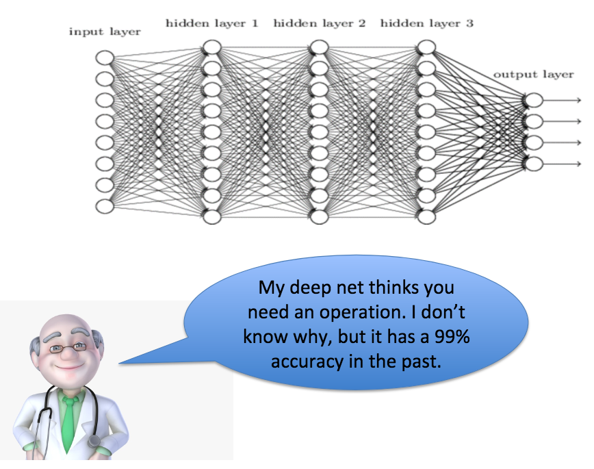
- Deep learning: recent methods that tries to solve some of the issues tackled above but using a black box.
Representative based
If we do not have enough information about users and items, we can rely more on those who “represent” the set of items and users. That’s the philosophy behind representative based methods.
Representatives can be users whose linear combinations of preferences accurately approximate other users’. For example, a famous representative based method, Representative Based Matrix Factorization (RBMF)1 is an extension of MF methods with an additional constraint that \(m\) items should be represented by a linear combination of \(k\) items, as can be seen from the objective function below:
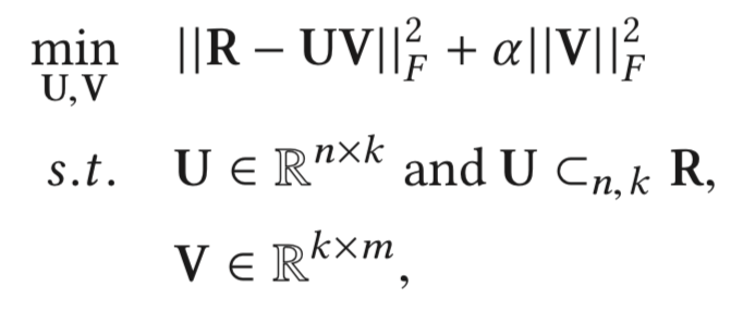
Here, we have the reconstruction error similar to standard MF methods, with this additional constraint. When a new user joins the platform, we can ask the new users to rate these \(k\) items, and use that to infer the ratings of other \(m-k\) items. This way, with a small additional cost on users of rating some items, we can improve the recommendations for new users.
There have been improvements on RBMF proposed, where we can interview only a subset of users instead of all the new users to decrease the burden on the new users2.
Advantages
- More interpretability, because new users can be expressed in terms of few representative items.
- If you’re using MF methods already, this can be a simple extension to handle cold start.
Disadvantages
- Need to change UI and front end logic to ask the users to rate the representative items.
Content Based
There are many side information that has been underutilized in recommendation systems. For example, citing one of the content based papers3 directly:
In recent years, the boundaries between e-commerce and social networking have become increasingly blurred. Many e-commerce websites support the mechanism of social login where users can sign on the websites using their social network identities such as their Facebook or Twitter accounts. Users can also post their newly purchased products on microblogs with links to the e-commerce product web pages.
As other examples, for recommending research papers on journal archives, we not only have the ratings but also the actual text of the paper available. We can incorporate these information as additional features for users to alleviate information scarcity for new users. For textual information, we can for example use LDA to obtain topic vectors for user posts. Even for social networks, there have been proposed a variety of graph embedding methods, which can represent graph nodes in vector spaces45.
How can we handle these contents in CF methods? Classic CF methods are essentially matrix completion with reconstruction error as its objective. Thus, it is hard to utilize these side information. Researchers have proposed hybrid methods that combines matrix reconstruction objective and content based objectives. These approaches are not cold start specific, so I’ll leave it to the readers to explore some literatures in depth 67.
Advantages
- Can incorporate a wide range of content information.
- Hybrid methods are extensions of MF.
Disadvantages
- Objective functions get cluttered. This is solved with deep methods, with a different downside.
- Lots of feature engineering? Depends on whether you have ready to plug-in user/item features in your db.
Bandit
Cold start can be reframed and solved as a bandit problem. What is a bandit problem? A classic example is the following: you are in a casino and you see \(k\) slot machines in front of you. Each slot machine has its own distribution of reward, but you do not have access to that information. Your goal is to maximize your return from playing these slot machines.
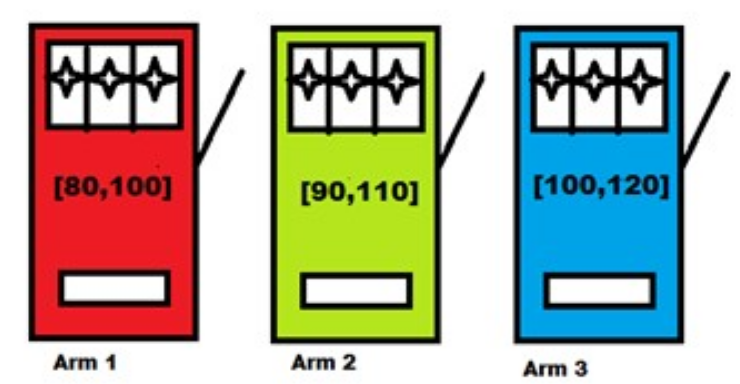
Why is this relevant? You can draw an analogy here. Think of an e-commerce problem where you have \(k\) new items arriving on your platform everyday. These \(k\) items can be thought of as slot machines with different returns (e.g. revenue, profit). But since they are new items, you do not have access to how much users will buy them. Then, recommending a subset of these items is like choosing a subset of slot machines to draw.
In bandit problems, we very much care about the exploration vs exploitation problem. If we found a new item that sells very well, we would like to show it to users more (exploitation). But at the same time, you would also want to show others which have not been shown as much, because they can be even more popular then the items you have shown already (exploration).
Solutions to the Bandit Problem
The bandit problem is well studied and there are many ways to solve this problem:
-
\(\epsilon\) greedy8: This is the simplest approach. Show an item that’s discovered to be most popular (e.g. highest average sales / clicks / views among users so far) with probability \(\epsilon\). Show a random item with \(1-\epsilon\). \(\epsilon\) controls whether to focus more on exploitation vs exploration.
-
Upper Confidence Bound (UCB)8: Select an item that maximizes \(\hat{\mu_j} + \sqrt{\frac{2\ln t}{t_j}}\). \(\mu_j\) is the average sales / clicks / views of item \(j\) so far. \(t\) is the number of times you’ve shown the new items. \(t_j\) is the number of times item \(j\) was shown. Clearly, \(\mu_j\) is the criteria for exploitation (e.g. favor items with more average sales) and \(\sqrt{\frac{2\ln t}{t_j}}\) for exploration (e.g. favor items with less exposure so far). This weird \(\log\) and \(\sqrt\) comes from the confidence interval of \(E[\mu_{i,j}]\), which you can read more about in this paper8.
-
Thompson Sampling (TS)9: Think of this as a Bayesian version of the approaches above. You define some prior (e.g. gaussian) with parameters, obtain some observations to calculate the likelihood, and then update the prior with the posterior. We can then choose an action that maximizes the reward based on the posterior distribution of the parameters.
Contextual Bandit
Contextual bandit problem is a generalization of the bandit problem that resembles real world cases more closely. The only difference now is that, in addition to the action (e.g. which items to show) and reward (e.g. sales), you now have contexts (e.g. item discription, pictures, the number of times it was clicked). By utilizing these contexts, we can have a better estimate of the reword. For example, in UCB above, we can add to the reward function a linear combination of the context features. In TS, we can have the likelihood function depend not only on the rewards and actions but also on the contexts.
Advantages
-
Easy to implement: The simple bandit algorithms are quite easy to implement, especially compared to sophisticated machine learning methods. So bandit methods are definitely a good baseline to compare to.
-
Nice theoretical guarantees: As ML practitioners, you might care little about theoretical guarantees, but thanks to its simplicity, a lot of theoretical analysis has been done on the average and the worst case reward. So you can be rest assured that the algorithms won’t be a disaster.
Disadvantages
- Too simple?: Maybe, maybe not. Bandit might just be good enough.
Deep Learning
I’m treating deep learning as one big category for tackling the cold start problem, but note that the ways deep learning is used in these papers are very diverse. There are many other recent methods that use deep learning. You might be able to find one that fits your context here10.
A simple trick used in Deep Learning based Youtube Recommendation
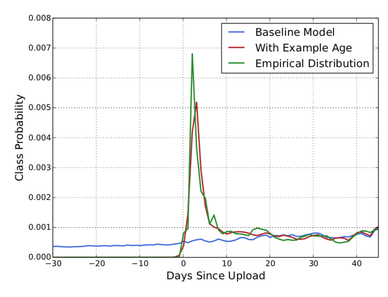
Deep Neural Networks for YouTube Recommendations11 is not specifically about cold start. Nonetheless, they recognize the cold start problem and proposes a simple hack to deal with it. Namely, among the many features on video watches, search tokens, geographic and biographic information, they included Days Since Upload. Training a deep network with this additional feature, they observed that their deep net learns that “fresh” videos are more important.
DropoutNet12:
The basic idea is simple yet powerful. Their approach is that, in training deep learning based recommendation systems (e.g. collaborative filtering with many layers), we can make it robust against the cold items by randomly dropping ratings of items and users. The key here is that, as opposed to standard dropout in neural net training, they drop the features, not the nodes. By doing so, they can make the neural net depend less on certain ratings, and be more generalizable to items/users with less ratings. The strength of their approach is that it can be used with any neural net based recommender systems, and also that the approach works for cold start in both users and items.
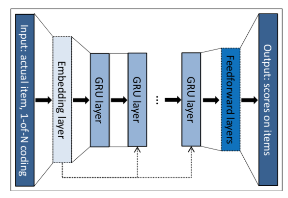
Session-based RNN13:
This approach tries to utilize each session of users by feeding it into an RNN. Specifically, they trained a variant of Gated Recurrent Unit (GRU), where the input is the current state of the session and the output is the item of the next event in the session. This networks is useful e.g. in smaller e-commerce sites where only a few user sessions are available.
Advantages
- If you can find a model for a specific domain that fits with your purpose nicely, you might boost the recommendation performance significantly.
Disadvantages
- Takes time to implement and tune the model.
- Deploying deep models can take more time, depending on your current stack.
- No guarantee on how well it will do.
Conclusion
Assuming you have some recommender system in place in your product, you want to find the solution to cold start that satisfies the following:
- Suitable for your domain.
- Can built on top of an existing system, or can be implemented and improved quickly.
For example, you can start from bandit and then move on to deep learning methods. In an industry environment, a model that might look too simple is always better. It is more maintainable, interpretable, and can be improved quickly.
I hope you found some good hints on how to get started on your cold start solution!
-
Wisdom of the Better Few: Cold Start Recommendation via Representative based Rating Elicitation ↩
-
Local Representative-Based Matrix Factorization for Cold-Start Recommendation ↩
-
Connecting Social Media to E-Commerce: Cold-Start Product Recommendation Using Microblogging Information ↩
-
SVDFeature: A Toolkit for Feature-based Collaborative Filtering ↩
-
Personalized recommendation via cross-domain triadic factorization ↩
-
Finite-time analysis of the multiarmed bandit problem ↩ ↩2 ↩3
-
Thompson Sampling for Contextual Bandits with Linear Payoffs ↩
-
Session-based Recommendations with Recurrent Neural Networks ↩