AI in Society: 1. Interpretability

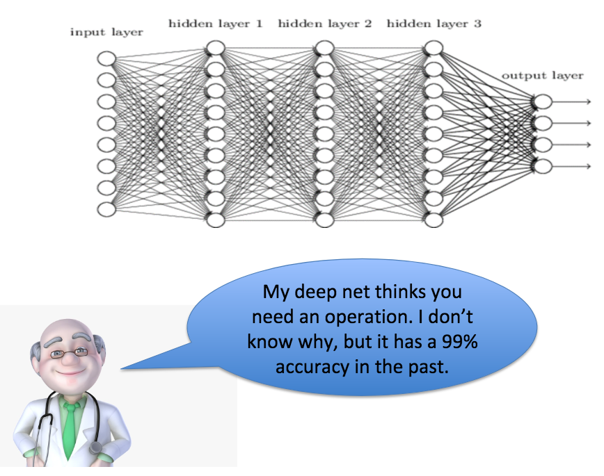
Would you believe in doctors that tell you this?

Another example. Consider a politician telling you “let’s implement this policy because my AI says it’s going to improve our country”. Would you vote for him/her?

If you are fine with these scenarios, go watch Netflix. If this is a bit disturbing, continue scrolling down.

In this post, I’ll introduce recent research for improving the interpretability of machine learning models. Interpretability is extremely hard to quantify and to optimize for. But this also means that the field is diverse, full of many interesting approaches to deal with black box models. Let’s take a look at some of them. Because this is a post on interpretability, I have lots of images and plots for you :) ¹

Early days: variable selection with L1 regularization

Research in interpretability of machine learning algorithms is not new. It has been studied for more than a decade. One of the early attempts to interpret machine learning was the invention of L1 regularization and L1 regularization paths. The basic idea is that L1 regularization induces sparsity in the set of variables used in a model, ending up in a more parsimonious model. The claim is that if the model has fewer variables, we can have better interpretability.

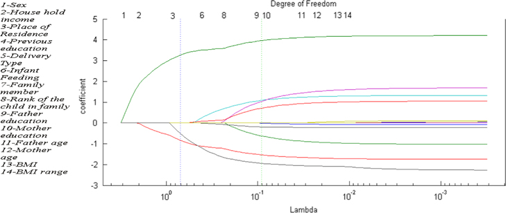
This is an image of an L1 regularization path ². On the x-axis, we have the strength of L1 regularization parameter \(\lambda\). Higher \(\lambda\) means more sparsity. On the y-axis, we have the value of coefficients for each feature. The lines represent how the feature coefficients change as we decrease \(\lambda\). As we can see, the higher \(\lambda\) is (left) the fewer the number of variables. We can also see when different variables kick in to the model as we lower \(\lambda\).

Then comes sparsity of samples

An orthogonal line of work that is a bit more recent is the idea of selecting a subset of data (“a prototype set”) which best covers the whole set of data classified by a certain label. These prototype sets can formally optimally found via a set cover integer program, which reflects how an idea prototype set should behave. For example,

• Every training example should have a prototype of its class as its neighborhood.
• No point should have a prototype of a different class as its neighborhood.
• The fewer the number of prototypes the better.

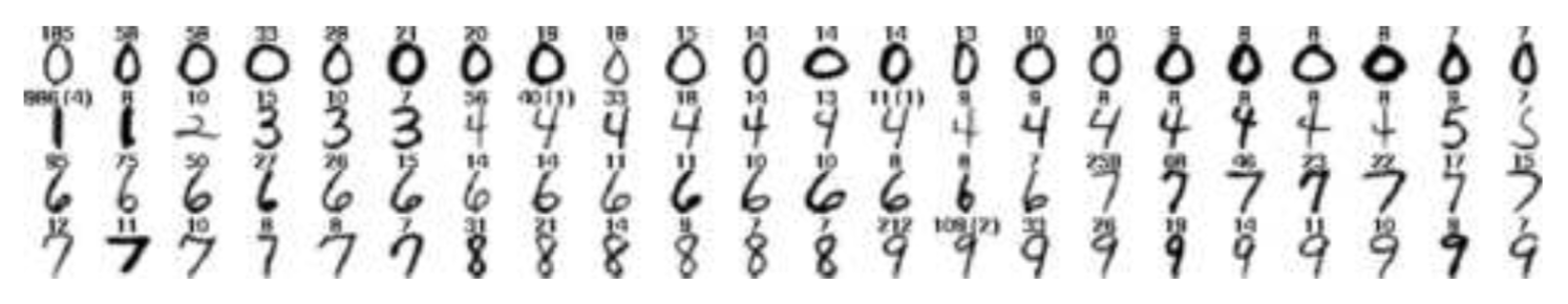
A greedy solution to this set-cover problem selects one image at a time as a prototype so as to maximize the increase in the number of other images correctly covered. The above image shows the first 88 prototypes for the MNIST data. It’s a bit hard to see, but the number on top of each MNIST image correspond to the number of images newly covered correctly by adding that image as a prototype. For example, for “1”, you need only two prototypes to explain the images, but for “7”, you need many more different prototypes.

For the actual formulation of the integer program, and details of the algorithm for solving it, you can refer to the original on prototype selection ³.

Decision Sets

If we can have a much more interpretable model with slightly less harm in accuracy, we might be better off using the simpler model instead. This is the idea behind decision sets ⁴. The basic idea is to learn a model that is almost as good as deep learning or other sophisticated models with a set of rules that are much simpler.

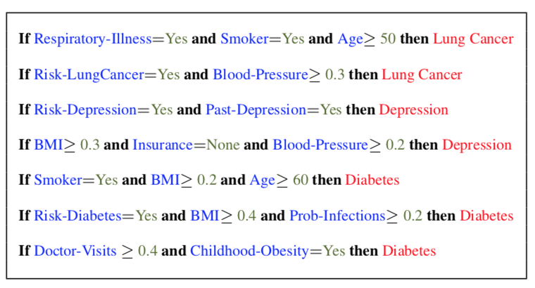
To find such rules, we need to have an objective function. The objective function should have two terms for accuracy and interpretability. Defining interpretability is hard, but the authors of decision sets paper consider things like the length of the rules (less is better), the set of data points covered by each rule (more is better), the overlap across different rules (less is better). Then, we can solve this using some optimization algorithm.

Scoring Systems

This one is perhaps the most widely used method for interpretable machine learning. It is so popular that it might not seem like machine learning at all. But I think scoring systems ⁵ are really cool because of its extreme simplicity.

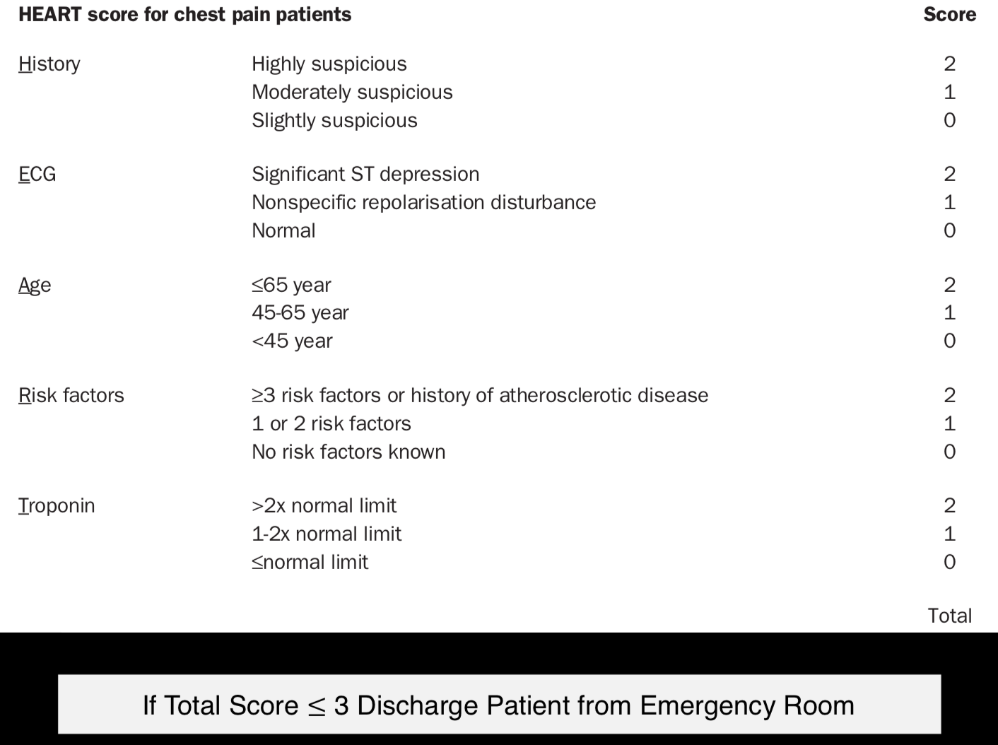
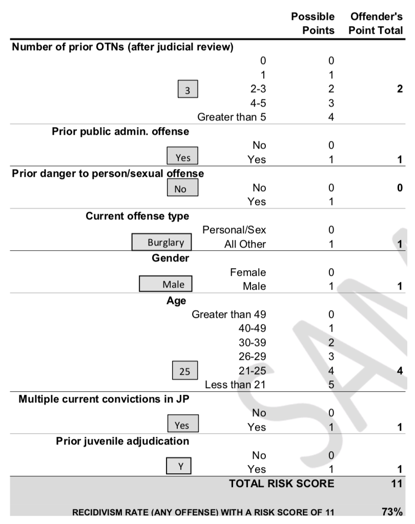
Have you seen a medical diagnosis test like this online? This is called a scoring system. I would assume that many of these you’ve encountered are suboptimal, but there is a rigorous optimization based approach behind constructing these scoring systems, and they are widely used in medical diagnosis, jurisdictional decision makings and more.

Given a dataset \((\mathbf{x}_1,y_1),...,(\mathbf{x}_n,y_n)\), we can make a prediction based on a linear combination of the features with the coefficients (scores) being small integers:

\[\hat{y}_i=+1 \text{ if } \lambda_1 x_{i,1}+\lambda_2 x_{i,2}+...+\lambda_d x_{i,d} > \lambda_0\]

where \(\lambda_0\) is some threshold for the total score, and \(\lambda_i \in \{-10,...,10\}\) or some other range of small integers. This is called a Supersparse Linear Integer Model (SLIM), and Ustun et al. have proposed ways to optimize this integer program quickly. The resulting \(\lambda_i\)’s then gets used in the scoring systems you often see.

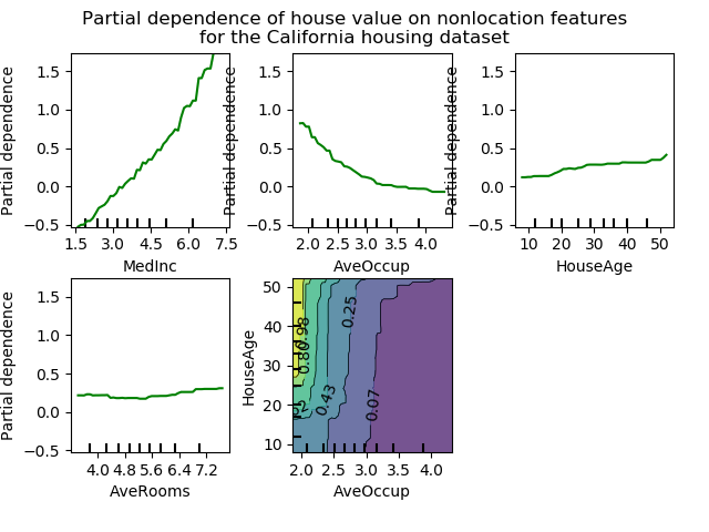
Being Causal

I put this in the end because I personally think this is the most important approach to interpretability of all. The idea behind these causal approaches is that we can best interpret black-box models if we know exactly what would’ve happened (1) if one feature changed, everything else held constant or (2) if one data point changed, everything else held constant. One widely used approach for (1) is the partial dependency plot (PDP). The definition of partial dependence is pretty simple. If you have a set of variables \(X\), and a subset \(X_S\) (with its complement \(X_C\)), a partial dependence of a machine learning model \(g(x)\) is defined as:

\[g_S(x_S)=E_{X_C}[g(x_S,X_c)]\]

The above formula basically marginalizes out the effect of other variables. It has been shown that PDP has a close connection to backdoor criterion, a notion in causal inference which all researchers in the domain are familiar with ⁶.

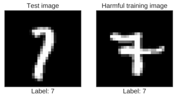
For (2), a recent paper ⁷ uses what is known as influence functions to answer “what would happen if we did not have this training point, or if the values of this training point were changed slightly?” I won’t describe the formal definition here, but the basic idea of influence function is that it approximates the parameter change of a model when an input was perturbed by a small amount. I intuitively understand this as looking at the change in model weights via something like a gradient descent with one input which we are interested in analyzing. With influence functions, we can for example know which train images are harming the classification of test examples the most:

Conclusion

I want to make three points before I end. There are two approaches to interpretability. One is to use a complex model (like deep nets), but have good tools to enhance it’s interpretability (e.g. influence functions). Another is to train inherently interpretable models to begin with (e.g. scoring systems, decision sets). Which approach is more suitable depends on different occasions.

Second, the fact that ML savvy people think that a model or an approach is interpretable does not imply that the general public, or the users of these models would think the same way. HCI type researches to verify whether claimed-to-be interpretable models are actually interpretable or useful for them are scarce ⁸. I hope that the research on interpretability should go in this direction.

Finally, you might have found these works less “sexier” than e.g. recent techniques in GAN being able to learn to generate celebrity images. But that’s kind of the whole point of research in interpretability. The goal is to demystify what people call “black box” or “machine intelligence” or even “magic”, and to represent what’s happening underneath the hood as vividly as possible. I believe that the “uncooler” we can think about machine learning, the more successful we are at interpreting what they are really doing.

1. Many of the papers and visualizations were introduced in COMPSCI 236R: Topics at the Interface between Computer Science and Economics, a course I took at Harvard in Spring 2018. Thank you Professor Chen! ↩

2. L1 Regularization Path Algorithm for Generalized Linear Models ↩

3. Prototype selection for interpretable classification ↩

4. Interpretable Decision Sets: A Joint Framework for. Description and Prediction ↩

5. Supersparse Linear Integer Models for Optimized Medical Scoring Systems ↩

6. Causal Interpretations of Black-Box Models ↩

7. Understanding Black-box Predictions via Influence Functions ↩

8. One of the very few is Manipulating and Measuring Model Interpretability ↩