SVD -> PCA

I wrote a blog about Robust PCA. As a prerequisite for the readers, I will explain what SVD and PCA are. As we shall see, PCA is essentially SVD, and learning these two will be a nice segue way to robust PCA.

SVD

Formula

Any matrix \(A \in \mathbb{R}^{m \times n}\) can be written as

\[A=U\Sigma V^\intercal\]

where \(U \in \mathbb{R}^{m \times m}\) is an orthogonal matrix,
\(V \in \mathbb{R}^{n \times n}\) is also an orthogonal matrix,
and \(\Sigma \in \mathbb{R}^{m \times n}\) is a diagonal matrix.

Diagonal values of \(\Sigma\) are called singular values. SVD shows that we can decompose any rectangular matrices into three matrices with nice properties (i.e. orthogonal and diagonal).

Low Rank SVD

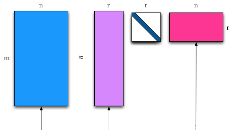
In machine learning, we use low rank (or truncated) SVD a lot, because it can compress the information \(A\) has to smaller matrices. Formally,

\[A\approx U_t\Sigma_t V_t^\intercal\]

where \(U_t \in \mathbb{R}^{m \times t}\) is an orthogonal matrix,
\(V_t \in \mathbb{R}^{t \times t}\) is also an orthogonal matrix,
and \(\Sigma_t \in \mathbb{R}^{t \times n}\) is a diagonal matrix.

\(\Sigma_t\) contains \(t\) largest singular values. The rows and columns in \(U_t,V_t\) can be thought of as “the most information rich” vectors of \(U,V\). Note that the exact equality no longer holds. Here is an image that illustrates the above formula:

Finding \(U\) and \(V\)

Recall that the definition of an orthogonal matrix is \(X^\intercal X=X X^\intercal=I\). Using this fact, you can find \(U,V\) by using eigen decomposition twice.

\[\begin{align} A^\intercal A&=(V\Sigma^\intercal U^\intercal) (U\Sigma V^\intercal) &\\ &=V(\Sigma^\intercal \Sigma)V^\intercal \end{align}\] \[\begin{align} A A^\intercal&=U(\Sigma^\intercal \Sigma)U^\intercal \end{align}\]

Essentially, applying eigen decomposition to \(A^\intercal A, A A^\intercal\) gives us \(V,U\) as stacks of eigen vectors. Eigen values in the diagonal entries of \(\Sigma^\intercal \Sigma\) correspond to the square of the singular values.

Applications

There are numerous applications of (truncated) SVD:

• Collaborative filtering is an algorithm for recommender systems. \(A\) is a user \(\times\) item matrix, which is decomposed into \(U_t\), a user matrix and \(V_t\) an item matrix. SVD finds a \(t\) dimensional embedding vector for each user and item.

• Image Compression: \(A\) is the original image. \(A\) can be decomposed into smaller matrix space by choosing a small \(t\). Below, you can see the reconstructed images for different values of \(t\). The lower the \(t\) is, the more compressed the image is. Image quality does go down, but it does preserve many important aspects of the original image.

• Semantic Indexing: What is known as LSI (latent semantic indexing) in NLP is essentially SVD. In LSI, \(A\) is a term frequency matrix of dimension document \(\times\) term. \(U_t,V_t\) are low dimensional embeddings of document, term, respectively.

PCA

I would say that PCA is one of the applications of SVD.

The objective of PCA is to “compress” a data matrix to a lower rank:

\[\min ||D-A|| \ s.t. \ rank(A) \leq t\]

Solving this optimization function let’s us find \(A\) with rank at most \(k\) that best approximates \(D\). Eckart and Young proved in 1936 ¹ (!) that the optimal \(A\) is \(X^t\), \(X\) with only the top \(t\) principal components. What are principal components? We already calculated them above! It’s \(U_t\Sigma_t\). Corresponding principal “principal vectors” are \(V_t\). PCA is that simple. This is true for all norms that are invariant under unitary transformations. To learn more about matrix norms, see this. We will be using some of them in Robust PCA.

Conclusion

I hope you see how PCA is easily derived from SVD. Now that you know PCA, you’re ready to learn Robust PCA!

1. The approximation of one matrix by another of lower rank ↩