Robust PCA

PCA is great because you can reduce a data matrix to a lower dimension without losing much. Although it is widely used, PCA doesn’t work well when there are noises in the input data. This is because the objective function \(\min \vert \vert D-A \vert \vert\) doesn’t really incorporate the fact that the input might be noisy. As the name suggests, Robust PCA is a variant of PCA that is more robust against noises. It was efficiently solved by Candès et al. in 2011¹.

*If you want a quick review on PCA, read my previous post and then come back.

Goal

The goal of Robust PCA is \(D=A+E\). This goal can be best illustrated with the image below:

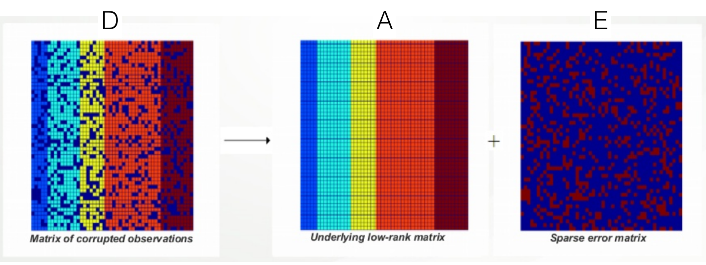
The intuition is that noisy images should be able to be decomposed into \(A\) (underlying less noisy image) and \(E\) (noise). Just like PCA, we would like \(A\) to be of lower rank. Furthermore, since \(E\) is a noise, we want it to be sparse.

Objective Function: PCP

How can we formulate this intuition in terms of an objective function? First thought would be to try this:

\[\begin{align} & \min_{A,E} \text{rank}(A) + \lambda \vert \vert E\vert \vert_0 & \\ & s.t. D=A+E \end{align}\]

The first terms ensures \(A\) is low rank and the second term ensures \(E\) is sparse. Note that \(\vert \vert E\vert \vert_0\) is the \(l_0\) norm, the number of non-zero elements in \(E\). If you’ve learned optimization before, you will know that this is not a good objective function. This is because the objective is neither continuous nor convex.

The key insight Candès provided in his paper is that we can proxy this with what he named Principal Component Pursuit (PCP):

\[\begin{align} & \min_{A,E} \vert \vert A \vert \vert_* + \lambda \vert \vert E\vert \vert_1 & \\ & s.t. D=A+E \end{align}\]

Lower rank is now enforced by the nuclear norm, which is essentially the sum of singular values of \(A\). Sparsity is enforced by the \(l_1\) norm, which I hope you’re familiar with.

Candès showed that this proxy optimization function has the following property:

If \(A\) is sufficiently low rank but not sparse AND \(E\) is sufficiently sparse but not low rank, then \(D\) can be recovered exactly with \(\lambda=\frac{1}{\sqrt{\max(m,n)}}\). (Theorem 1.1)

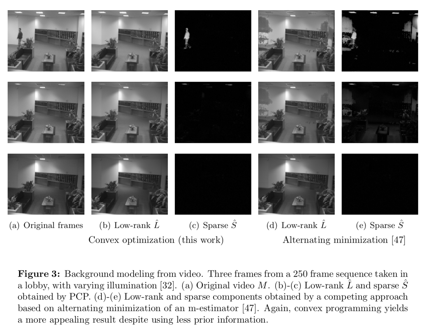
This is amazing, because decomposing \(D\) into \(A\) and \(E\) in an unsupervised fashion seems very very hard. The theorem states that this is possible. Section 2 and 3 of his paper proves this theorem. Section 4 empirically shows that PCP can reconstruct. I will not cover these sections in this post, but I’ll leave a picture of the experimental result from the original paper here:

How to Solve PCP

PCP is convex, so we can solve it for example using interior point methods. However, the author claims that this is not fast enough (with \(O(n^6)\) run time). In section 5, he introduces augmented Lagrange multiplier (ALM), which I found is interesting.

ALM

Before discussing how we can solve PCP, let’s briefly learn what ALM does. Say we have the following optimization problem:

\[\begin{align} & \min_{\mathbf{x}} f(\mathbf{x}) & \\ & s.t. c_j(\mathbf{x})=0, j\in [m] \end{align}\]

There are two ways to solve this:

1. Langrange multiplier

We can reformualte the above problem using a Langrange multipler \(\lambda_j\) and solve instead:

\[\min_{\mathbf{x}} f(\mathbf{x}) + \sum_{j=1}^m c_j(\mathbf{x})\]

2. Penalty method

A less known approach is called the penalty method. The basic idea is that we can solve the above objective function by solving repeatedly

\[\min_{\mathbf{x}} f(\mathbf{x}) + \mu \sum_{j=1}^m c_j^2(\mathbf{x})\]

Here, we are using a quadratic loss function \(c_j^2(\mathbf{x})\), but it can be linear, cubed, anything. The algorithm is as follows:

1. Solve this optimization problem.
2. Increment \(\mu=\rho \mu\). (\(\rho=10\) is commonly used).
3. Solve the next optimization problem starting from \(\mathbf{x}^*\) from the previous step.
4. Repeat until convergence.

ALM = Langrange + Penalty Method

ALM basically combines these two by iteratively solving the following, updating \(\mu\) each iteration until convergence:

\[\min_{\mathbf{x}} f(\mathbf{x}) + \sum_{j=1}^m c_j(\mathbf{x}) + \frac{\mu}{2} \sum_{j=1}^m c_j^2(\mathbf{x})\]

PCP as ALM

Now, we can formulate PCP in ALM form using matrix notations:

\[\min_{A,E} \vert \vert A \vert \vert_* + \lambda \vert \vert E\vert \vert_1 + \langle Y,D-A-E \rangle + \frac{\mu}{2} \vert \vert D-A-E \vert \vert^2_F\]

where F is the Frobenius norm (square root of the sum of squares of matrix elements) and \(Y\) is the lagrange multipliers.

In practice, we need to alternately optimize \(A,E\). Closed form update formula for these are quite straightforward to derive.

Conclusion

Robust PCA is regarded as one of the master pieces in machine learning papers. I skipped the proof of theorem 1.1 entirely, but I hope you at least got the gist of what it is optimizing for, and how it is done.

1. Robust PCA ↩